Atlantic Multidecadal Variability

Background

Atlantic Multidecadal Variability (AMV), also known as Atlantic Multidecadal Oscillation (AMO), is a climate phenomenon characterized by multidecadal fluctuations in sea surface temperatures (SSTs) in the North Atlantic (Fig. 1). These variations typically occur on timescales of about 50-80 years and can have significant impacts on regional and global scales.

The driver of the Atlantic Multidecadal Variability (AMV) remains unclear, despite its significance. Various factors are believed to contribute to its variability. One key factor is the Atlantic Meridional Overturning Circulation (AMOC), a planetary-scale ocean circulation that transports energy from the Southern Hemisphere to the Northern Hemisphere. Changes in the AMOC naturally result in variability in the sea surface temperatures (SST) in the North Atlantic (Zhang et al., 2019). Although the role of the AMOC has been verified in numerous climate model simulations, direct measurements of AMOC intensity only began in the 2000s, providing insufficient data to conclusively verify this hypothesis.

High-frequency atmospheric variability could also lead to low-frequency AMV. Clement et al. (2015) used a model with a slab ocean to demonstrate that the North Atlantic Oscillation (NAO) can induce the AMV pattern without involving ocean dynamics like the AMOC. However, this has been critiqued by several studies (see comment papers on the topic). The study of atmospheric contributions to the AMV remains an active research area, gaining increasing recognition within the scientific community. Nevertheless, the AMOC argument still appears to be the most favored.

Lastly, external forcings such as volcanic eruptions, solar variability, and anthropogenic aerosols could also drive the AMV. To my knowledge, this idea was first proposed in a “commentary” paper published in EOS by Michael Mann and Kerry Emanuel (2006). However, the concept did not gain widespread acceptance until an influential paper by Booth et al. (2012) was published in Nature. Booth et al. (2012) successfully replicated the AMV using the Met Office climate model, suggesting that anthropogenic aerosols were the primary drivers of the AMV over the past century. This seemed to resolve the debate, as their simulation indicated that the AMV could not exist without anthropogenic aerosol emissions. However, a year later, researchers from the Geophysical Fluid Dynamics Laboratory (GFDL) reanalyzed Booth’s simulation and raised concerns about the model’s aerosol effect, which was found to be strongly biased and inconsistent with real-world observations (Zhang et al., 2013). Despite this, the idea of external forcing had taken root in the scientific community, leading to further studies emphasizing its role, although the AMOC remains the more popular explanation.

Progress

Over the past decade, large ensemble historical simulations have emerged, helping the community gain a better understanding of the roles played by external forcing and internal variability. The consensus is that the AMV comprises both internal and external variability, with the internal component being dominant (e.g., Qin et al., 2021). This conclusion is based on the dramatic difference between the modeled forced AMV and observations, particularly the much smaller modeled response, implying that the real-world AMV is internally driven. However, some researchers disagree. They argue that the correlation between the modeled forced AMV and observations is actually quite high—exceeding 0.8 since 1950 (e.g., Bellomo et al., 2017; Murphy et al., 2017, 2021; Kalavans et al., 2022)—despite the anemic forced response. This suggests the opposite: that the real-world AMV is mostly forced, and the weak response in models is due to a bias known as the signal-to-noise problem.

My answer

While focusing solely on the AMV time series is helpful, it cannot resolve the debate, much like trying to determine someone’s family based on appearance alone. Similar looks do not necessarily indicate familial ties, and differences do not preclude them. What truly matters is their DNA.

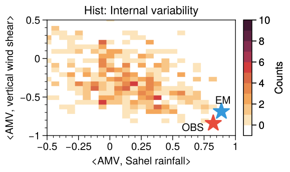
So, what is the DNA of the AMV? Inspired by Yan et al. (2017), my recent study offers a crucial DNA marker for identifying the origin of the AMV. We examined the correlation between the AMV and its impacts, such as Atlantic hurricanes and Sahel rainfall. These correlations are independent of the evolving trajectories and magnitudes of the AMV, relying solely on their coupled dynamics. If the real world were driven by internal variability, the observed “DNA” should resemble that found in modeled internal variability. In other words, the dynamics in the real world and internal variability are similar.

Fig. 2 illustrates the correlation between Sahel rainfall/vertical wind shear in the tropical Atlantic (a proxy for hurricane activity) and the AMV from 1950 to 2014. The observed correlation is approximately 0.85 (red star), whereas the correlations in modeled internal variability (shading) are significantly lower. Only a few model members come close to the observed correlation, and none exceed it. This indicates that internal variability and the real world do not share the same DNA. The likelihood of internal variability producing an AMV-Sahel rainfall-Atlantic hurricane system is extremely low—less than 2% (see Extended Data Fig. 5 of He et al., 2023). In contrast, the forced response (blue star) closely matches the observed value, suggesting that the real world is predominantly influenced by forced responses.

Will the scientific community accept that the AMV has been mostly forced since 1950? I hope so, but it seems unlikely. The pushback I received questioned the weak forced response in the model simulation, despite the fact that not only is the DNA of the forced response similar to the real world, but the time series of forced AMV, hurricane activity, and Sahel rainfall are also highly correlated with observations (see Fig. 2 in He et al., 2023). The weak forced response is indeed a problem, but it is distinct—the so-called signal-to-noise problem. Why is the modeled forced response so small, and why is the signal-to-noise ratio in the model so low? A problem has to be investigated.