R package to compute statistics from the American Community Survey (ACS) and Decennial US Census
The acsr package helps extracting variables and computing statistics using the America Community Survey and Decennial US Census. It was created for the Applied Population Laboratory (APL) at the University of Wisconsin-Madison.
Installation
The functions depend on the acs and data.table packages, so it is necessary to install then before using acsr. The acsr package is hosted on a github repository and can be installed using devtools:
devtools::install_github("sdaza/acsr")
library(acsr)
Remember to set the ACS API key, to check the help documentation and the default values of the acsr functions.
api.key.install(key="*")
?sumacs
?acsdata
The default dataset is acs, the level is state (Wisconsin, state = "WI"), the endyear is 2014, and the confidence level to compute margins of error (MOEs) is 90%.
Levels
The acsr functions can extract all the levels available in the acs package. The table below shows the summary and required levels when using the acsdata and sumacs functions:
| summary number | levels |
|---|---|
| 010 | us |
| 020 | region |
| 030 | division |
| 040 | state |
| 050 | state, county |
| 060 | state, county, county.subdivision |
| 140 | state, county, tract |
| 150 | state, county, tract, block.group |
| 160 | state, place |
| 250 | american.indian.area |
| 320 | state, msa |
| 340 | state, csa |
| 350 | necta |
| 400 | urban.area |
| 500 | state, congressional.district |
| 610 | state, state.legislative.district.upper |
| 620 | state, state.legislative.district.lower |
| 795 | state, puma |
| 860 | zip.code |
| 950 | state, school.district.elementary |
| 960 | state, school.district.secondary |
| 970 | state, school.district.unified |
Getting variables and statistics
We can use the sumacs function to extract variable and statistics. We have to specify the corresponding method (e.g., proportion or just variable), and the name of the statistic or variable to be included in the output.
sumacs(formula = c("(b16004_004 + b16004_026 + b16004_048 / b16004_001)", "b16004_026"),
        varname = c("mynewvar", "myvar"),
        method = c("prop", "variable"),
        level = c("division"))
## [1] "Extracting data from: acs 2014"
## [1] ". . . . . . ACS/Census variables : 4"
## [1] ". . . . . . Levels : 1"
## [1] ". . . . . . New variables : 2"
## [1] ". . . . . . Getting division data"
## [1] ". . . . . . Creating variables"
## [1] ". . . . . . 50%"
## [1] ". . . . . . 100%"
## [1] ". . . . . . Formatting output"## sumlevel geoid division mynewvar_est mynewvar_moe myvar_est myvar_moe
## 1: 030 NA 1 0.0762 0.000347 770306 3490
## 2: 030 NA 2 0.1182 0.000278 3332150 9171
## 3: 030 NA 3 0.0599 0.000196 1819417 7209
## 4: 030 NA 4 0.0411 0.000277 547577 4461
## 5: 030 NA 5 0.1108 0.000246 4526480 11869
## 6: 030 NA 6 0.0320 0.000265 402475 3781
## 7: 030 NA 7 0.2203 0.000469 5318126 13044
## 8: 030 NA 8 0.1582 0.000602 2279303 10746
## 9: 030 NA 9 0.2335 0.000501 7765838 20289To download the data can be slow, especially when many levels are being used (e.g., blockgroup). A better approach in those cases is, first, download the data using the function acsdata , and then use them as input.
mydata <- acsdata(formula = c("(b16004_004 + b16004_026 + b16004_048 /  b16004_001)",
        "b16004_026"),
        level = c("division"))
## [1] ". . . . . . Getting division data"sumacs(formula = c("(b16004_004 + b16004_026 + b16004_048 / b16004_001)", "b16004_026"),
varname = c("mynewvar", "myvar"),
method = c("prop", "variable"),
level = c("division"),
data = mydata)## [1] "Extracting data from: acs 2014"
## [1] ". . . . . . ACS/Census variables : 4"
## [1] ". . . . . . Levels : 1"
## [1] ". . . . . . New variables : 2"
## [1] ". . . . . . Creating variables"
## [1] ". . . . . . 50%"
## [1] ". . . . . . 100%"
## [1] ". . . . . . Formatting output"## sumlevel geoid division mynewvar_est mynewvar_moe myvar_est myvar_moe
## 1: 030 NA 1 0.0762 0.000347 770306 3490
## 2: 030 NA 2 0.1182 0.000278 3332150 9171
## 3: 030 NA 3 0.0599 0.000196 1819417 7209
## 4: 030 NA 4 0.0411 0.000277 547577 4461
## 5: 030 NA 5 0.1108 0.000246 4526480 11869
## 6: 030 NA 6 0.0320 0.000265 402475 3781
## 7: 030 NA 7 0.2203 0.000469 5318126 13044
## 8: 030 NA 8 0.1582 0.000602 2279303 10746
## 9: 030 NA 9 0.2335 0.000501 7765838 20289Standard errors
When computing statistics there are two ways to define the standard errors:
- Including all standard errors of the variables used to compute a statistic (
one.zero = FALSE) - Include all standard errors except those of variables that are equal to zero. Only the maximum standard error of the variables equal to zero is included (
one.zero = TRUE) - The default value is
one.zero = TRUE
For more details about how standard errors are computed for proportions, ratios and aggregations look at A Compass for Understanding and Using American Community Survey Data.
Below an example when estimating proportions and using one.zero = FALSE:
sumacs(formula = "(b16004_004 + b16004_026 + b16004_048) / b16004_001",
            varname =  "mynewvar",
            method = "prop",
            level = "tract",
            county = 1,
            tract = 950501,
            endyear = 2013,
            one.zero = FALSE)
## [1] "Extracting data from: acs 2013"
## [1] ". . . . . . ACS/Census variables : 4"
## [1] ". . . . . . Levels : 1"
## [1] ". . . . . . New variables : 1"
## [1] ". . . . . . Getting tract data"
## [1] ". . . . . . Creating variables"
## [1] ". . . . . . 100%"
## [1] ". . . . . . Formatting output"## sumlevel geoid st_fips cnty_fips tract_fips mynewvar_est mynewvar_moe
## 1: 140 55001950501 55 1 950501 0.0226 0.0252When one.zero = TRUE:
sumacs(formula = "(b16004_004 + b16004_026 + b16004_048) / b16004_001",
            varname = "mynewvar",
            method = "prop",
            level = "tract",
            county = 1,
            tract = 950501,
            endyear = 2013,
            one.zero = TRUE)
## [1] "Extracting data from: acs 2013"
## [1] ". . . . . . ACS/Census variables : 4"
## [1] ". . . . . . Levels : 1"
## [1] ". . . . . . New variables : 1"
## [1] ". . . . . . Getting tract data"
## [1] ". . . . . . Creating variables"
## [1] ". . . . . . 100%"
## [1] ". . . . . . Formatting output"## sumlevel geoid st_fips cnty_fips tract_fips mynewvar_est mynewvar_moe
## 1: 140 55001950501 55 1 950501 0.0226 0.0245When the square root value in the standard error formula doesn’t exist (e.g., the square root of a negative number), the ratio formula is instead used. The ratio adjustment is done variable by variable .
It can also be that the one.zero option makes the square root undefinable. In those cases, the function uses again the ratio formula to compute standard errors. There is also a possibility that the standard error estimates using the ratio formula are higher than the proportion estimates without the one.zero option.
Decennial Data from the US Census
Let’s get the African American and Hispanic population by state. In this case, we don’t have any estimation of margin of error.
sumacs(formula = c("p0080004", "p0090002"),
            method = "variable",
            dataset = "sf1",
            level = "state",
            state = "*",
            endyear = 2010)
## [1] "Extracting data from: sf1 2010"
## [1] ". . . . . . ACS/Census variables : 2"
## [1] ". . . . . . Levels : 1"
## [1] ". . . . . . New variables : 2"
## [1] ". . . . . . Getting state data"
## [1] ". . . . . . Creating variables"
## [1] ". . . . . . 50%"
## [1] ". . . . . . 100%"
## [1] ". . . . . . Formatting output"## sumlevel geoid st_fips p0080004 p0090002
## 1: 040 01 01 1251311 185602
## 2: 040 02 02 23263 39249
## 3: 040 04 04 259008 1895149
## 4: 040 05 05 449895 186050
## 5: 040 06 06 2299072 14013719
## 6: 040 08 08 201737 1038687
## 7: 040 09 09 362296 479087
## 8: 040 10 10 191814 73221
## 9: 040 11 11 305125 54749
## 10: 040 12 12 2999862 4223806
## 11: 040 13 13 2950435 853689
## 12: 040 15 15 21424 120842
## 13: 040 16 16 9810 175901
## 14: 040 17 17 1866414 2027578
## 15: 040 18 18 591397 389707
## 16: 040 19 19 89148 151544
## 17: 040 20 20 167864 300042
## 18: 040 21 21 337520 132836
## 19: 040 22 22 1452396 192560
## 20: 040 23 23 15707 16935
## 21: 040 24 24 1700298 470632
## 22: 040 25 25 434398 627654
## 23: 040 26 26 1400362 436358
## 24: 040 27 27 274412 250258
## 25: 040 28 28 1098385 81481
## 26: 040 29 29 693391 212470
## 27: 040 30 30 4027 28565
## 28: 040 31 31 82885 167405
## 29: 040 32 32 218626 716501
## 30: 040 33 33 15035 36704
## 31: 040 34 34 1204826 1555144
## 32: 040 35 35 42550 953403
## 33: 040 36 36 3073800 3416922
## 34: 040 37 37 2048628 800120
## 35: 040 38 38 7960 13467
## 36: 040 39 39 1407681 354674
## 37: 040 40 40 277644 332007
## 38: 040 41 41 69206 450062
## 39: 040 42 42 1377689 719660
## 40: 040 44 44 60189 130655
## 41: 040 45 45 1290684 235682
## 42: 040 46 46 10207 22119
## 43: 040 47 47 1057315 290059
## 44: 040 48 48 2979598 9460921
## 45: 040 49 49 29287 358340
## 46: 040 50 50 6277 9208
## 47: 040 51 51 1551399 631825
## 48: 040 53 53 240042 755790
## 49: 040 54 54 63124 22268
## 50: 040 55 55 359148 336056
## 51: 040 56 56 4748 50231
## 52: 040 72 72 461498 3688455
## sumlevel geoid st_fips p0080004 p0090002Output
The output can be formatted using a wide or long format:
sumacs(formula = "(b16004_004 + b16004_026 + b16004_048 / b16004_001)",
            varname = "mynewvar",
            method = "prop",
            level = "division",
            format.out = "long")
## [1] "Extracting data from: acs 2014"
## [1] ". . . . . . ACS/Census variables : 4"
## [1] ". . . . . . Levels : 1"
## [1] ". . . . . . New variables : 1"
## [1] ". . . . . . Getting division data"
## [1] ". . . . . . Creating variables"
## [1] ". . . . . . 100%"
## [1] ". . . . . . Formatting output"## geoid sumlevel division var_name est moe
## 1: NA 030 1 mynewvar 0.0762 0.000347
## 2: NA 030 2 mynewvar 0.1182 0.000278
## 3: NA 030 3 mynewvar 0.0599 0.000196
## 4: NA 030 4 mynewvar 0.0411 0.000277
## 5: NA 030 5 mynewvar 0.1108 0.000246
## 6: NA 030 6 mynewvar 0.0320 0.000265
## 7: NA 030 7 mynewvar 0.2203 0.000469
## 8: NA 030 8 mynewvar 0.1582 0.000602
## 9: NA 030 9 mynewvar 0.2335 0.000501And it can also be exported to a csv file:
sumacs(formula = "(b16004_004 + b16004_026 + b16004_048 / b16004_001)",
            varname = "mynewvar",
            method = "prop",
            level = "division",
            file = "myfile.out")
## [1] "Extracting data from: acs 2014"
## [1] ". . . . . . ACS/Census variables : 4"
## [1] ". . . . . . Levels : 1"
## [1] ". . . . . . New variables : 1"
## [1] ". . . . . . Getting division data"
## [1] ". . . . . . Creating variables"
## [1] ". . . . . . 100%"
## [1] ". . . . . . Formatting output"
## [1] "Data exported to a CSV file! "Combining geographic levels
We can combine geographic levels using two methods: (1) sumacs and (2) combine.output. The first one allows only single combinations, the second multiple ones.
If I want to combine two states (e.g., Wisconsin and Minnesota) I can use:
sumacs("(b16004_004 + b16004_026 + b16004_048 / b16004_001)",
    varname = "mynewvar",
    method = "prop",
    level = "state",
    state = list("WI", "MN"),
    combine = TRUE,
    print.levels = FALSE)
## [1] "Extracting data from: acs 2014"
## [1] ". . . . . . ACS/Census variables : 4"
## [1] ". . . . . . Levels : 1"
## [1] ". . . . . . New variables : 1"
## [1] ". . . . . . Getting combined data"
## [1] ". . . . . . Creating variables"
## [1] ". . . . . . 100%"
## [1] ". . . . . . Formatting output"## geoid combined_group mynewvar_est mynewvar_moe
## 1: NA aggregate 0.042 0.000331If I want to put together multiple combinations (e.g., groups of states):
combine.output("(b16004_004 + b16004_026 + b16004_048 / b16004_001)",
varname = "mynewvar",
method = "prop",
level = list("state", "state"),
state = list( list("WI", "MN"), list("CA", "OR")), # nested list
combine.names = c("WI+MN", "CA+OR"),
print.levels = FALSE)## [1] ". . . . . . Defining WI+MN"
## [1] "Extracting data from: acs 2014"
## [1] ". . . . . .  ACS/Census variables : 4"
## [1] ". . . . . .  Levels : 1"
## [1] ". . . . . .  New variables : 1"
## [1] ". . . . . .  Getting combined data"
## [1] ". . . . . .  Creating variables"
## [1] ". . . . . .  100%"
## [1] ". . . . . .  Formatting output"
## [1] ". . . . . . Defining CA+OR"
## [1] "Extracting data from: acs 2014"
## [1] ". . . . . . ACS/Census variables : 4"
## [1] ". . . . . . Levels : 1"
## [1] ". . . . . . New variables : 1"
## [1] ". . . . . . Getting combined data"
## [1] ". . . . . . Creating variables"
## [1] ". . . . . . 100%"
## [1] ". . . . . . Formatting output"## combined_group mynewvar_est mynewvar_moe
## 1: WI+MN 0.042 0.000331
## 2: CA+OR 0.269 0.000565A map?
Let’s color a map using poverty by county:
pov <- sumacs(formula = "b17001_002 / b17001_001 * 100",
        varname = c("pov"),
        method = c("prop"),
        level = c("county"),
        state = "*")
## [1] "Extracting data from: acs 2014"
## [1] ". . . . . . ACS/Census variables : 2"
## [1] ". . . . . . Levels : 1"
## [1] ". . . . . . New variables : 1"
## [1] ". . . . . . Getting county data"
## [1] ". . . . . . Creating variables"
## [1] ". . . . . . 100%"
## [1] ". . . . . . Formatting output"library(choroplethr)
library(choroplethrMaps)
pov[, region := as.numeric(geoid)]
setnames(pov, "pov_est", "value")
county_choropleth(pov, num_colors = 5)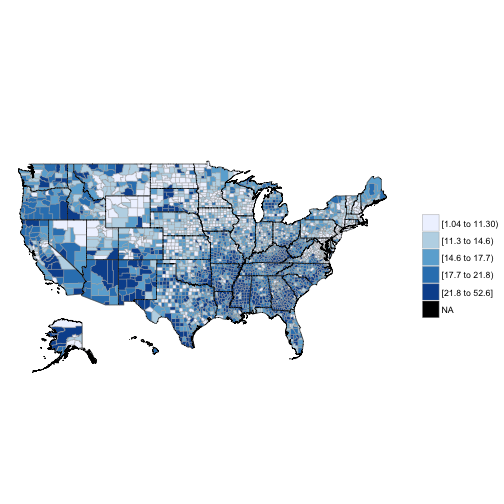
In sum, the acsr package:
- Reads formulas directly and extracts any ACS/Census variable
- Provides an automatized and tailored way to obtain indicators and MOEs
- Allows different outputs’ formats (wide and long, csv)
- Provides an easy way to adjust MOEs to different confidence levels
- Includes a variable-by-variable ratio adjustment of standard errors
- Includes the zero-option when computing standard errors for proportions, ratios, and aggregations
- Combines geographic levels flexibly
Last Update: 02/07/2016